16  MTT Analysis

Note

This protocol assumes you have finished the MTT Protocol.

This protocol also requires you have installed R, RStudio, as well as the mop and bladdr package. bladdr is a GitHub package. Use devtools::install_github("McConkeyLab/bladdr") to install bladdr and devtools::install_github("KaiAragaki/mop") to install mop. For more information, see ‘Installing GitHub Packages’.

16.1 Data Acquisition

  1. In the Spectramax software, click ‘File > Import/Export > Export…’ and export the results as a .txt file to a USB drive

16.2 Reading Data into R

  1. Open RStudio
  2. Press Shift + Ctrl/Command + N. This will open a new script.
  3. Run the following in your script, with the path to your file replacing the "dummy_mtt_spectramax.txt"
library(bladdr)
library(mop)

my_spectramax <- read_spectramax("dummy_mtt_spectramax.txt")
Please wait. This will take ~10 seconds.
Warning in grepl("^\t*$", lines): unable to translate ' Temperature(<a1>C) 1 2
3 4 5 6 7 8 9 10 11 12 1 2 3 4 5 6 7 8 9 10 11 12 ' to a wide string
Warning in grepl("^\t*$", lines): input string 3 is invalid
Warning in grepl("^\t*$", lines): unable to translate 'Copyright <a9> 2003
Molecular Devices. All rights reserved.' to a wide string
Warning in grepl("^\t*$", lines): input string 15 is invalid

You should now have a spectramax object that looks like this:

<spectramax[5]>
[[1]]
[[1]]$data

                12
   ________________________
  | ◯ ◯ ◯ ◯ ◯ ◯ ◯ ◯ ◯ ◯ ◯ ◯
  | ◯ ◯ ◯ ◯ ◯ ◯ ◯ ◯ ◯ ◯ ◯ ◯
  | ◯ ◯ ◯ ◯ ◯ ◯ ◯ ◯ ◯ ◯ ◯ ◯
  | ◯ ◯ ◯ ◯ ◯ ◯ ◯ ◯ ◯ ◯ ◯ ◯
8 | ◯ ◯ ◯ ◯ ◯ ◯ ◯ ◯ ◯ ◯ ◯ ◯
  | ◯ ◯ ◯ ◯ ◯ ◯ ◯ ◯ ◯ ◯ ◯ ◯
  | ◯ ◯ ◯ ◯ ◯ ◯ ◯ ◯ ◯ ◯ ◯ ◯
  | ◯ ◯ ◯ ◯ ◯ ◯ ◯ ◯ ◯ ◯ ◯ ◯
Start corner: tl
Plate dimensions: 8 x 12

[[1]]$type
[1] "Plate"

[[1]]$wavelengths
[1] "562" "660"


# Wavelengths: 562 
# Is tidy: TRUE 
# Date: 2023-09-14 

Now we need to calculate the proper values for plotting. This means we need to annotate our plate with our experimental conditions. To do this, we use mtt_calc.

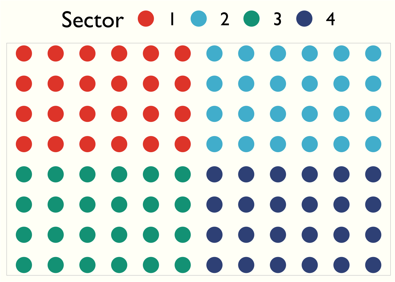
mtt_calc takes three arguments. One is the my_spectramax you just created. The second is the names of the conditions of each ‘sector’ of your plate. The third is the drug concentrations within that sector.

The order of sectors can be seen in Figure 16.1.

Figure 16.1: Order of sector labelling in the condition_names argument

In my data, I know I only used two sectors - sector 1 and 2.

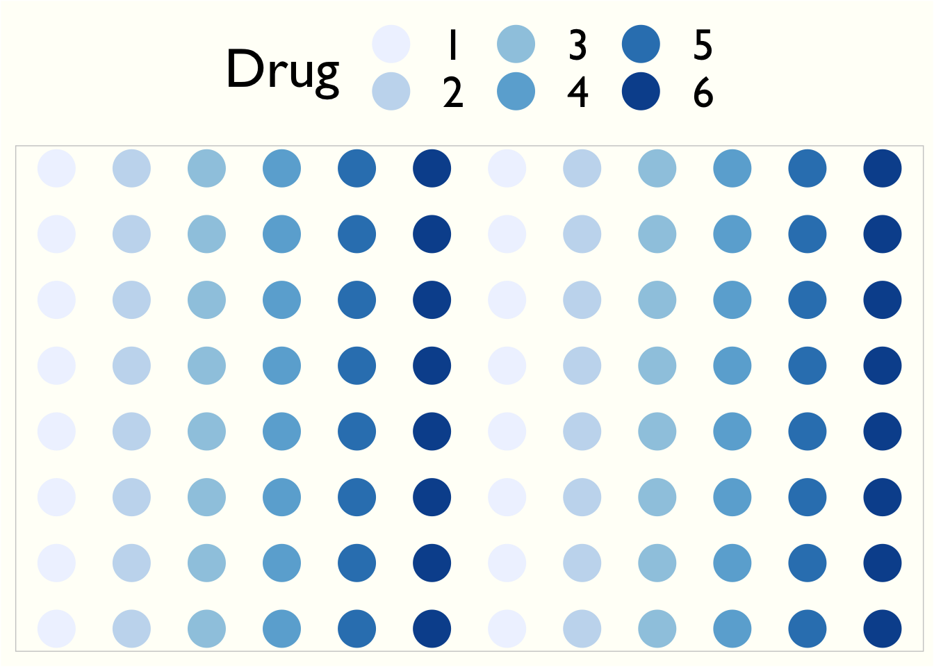
Additionally, you need to annotate the concentration of drug. It all needs numeric - not text - so it needs to be the same units. Additionally, it moves from left to right in each sector (see Figure 16.2).

Figure 16.2: Order of drug concentration labelling in the drug_conc argument

All this being said, here’s how I’ll annotate my plate:

my_mtt_calc <- mtt_calc(
  my_spectramax, 
  condition_names = c("Drug 1", "Drug 2", NA, NA),
  drug_conc = c(0, 1, 10, 100, 1000, 10000)
)
Lowest drug concentration is 0, converting to 1e-04
Warning: There were 2 warnings in `dplyr::mutate()`.
The first warning was:
ℹ In argument: `fit = purrr::map(.data$data, mtt_model)`.
ℹ In group 1: `condition = Drug 1`.
Caused by warning in `optim()`:
! method L-BFGS-B uses 'factr' (and 'pgtol') instead of 'reltol' and 'abstol'
ℹ Run `dplyr::last_dplyr_warnings()` to see the 1 remaining warning.
my_mtt_calc
# A tibble: 48 × 13
   condition  .row  .col nm562  nm660    drug   diff   mean   div fit   ic_value
   <fct>     <int> <dbl> <dbl>  <dbl>   <dbl>  <dbl>  <dbl> <dbl> <lis>    <dbl>
 1 Drug 1        1     1 0.494 0.0636  0.0001 0.430  0.410  1.05  <drc>    0.951
 2 Drug 1        2     1 0.471 0.0655  0.0001 0.405  0.410  0.988 <drc>    0.951
 3 Drug 1        3     1 0.462 0.066   0.0001 0.396  0.410  0.964 <drc>    0.951
 4 Drug 1        4     1 0.460 0.0504  0.0001 0.410  0.410  0.998 <drc>    0.951
 5 Drug 1        1     2 0.307 0.0538  1      0.253  0.227  0.618 <drc>    0.951
 6 Drug 1        2     2 0.292 0.0556  1      0.236  0.227  0.576 <drc>    0.951
 7 Drug 1        3     2 0.254 0.0523  1      0.202  0.227  0.493 <drc>    0.951
 8 Drug 1        4     2 0.259 0.0429  1      0.216  0.227  0.526 <drc>    0.951
 9 Drug 1        1     3 0.138 0.0446 10      0.0931 0.0854 0.227 <drc>    0.951
10 Drug 1        2     3 0.135 0.0478 10      0.0872 0.0854 0.213 <drc>    0.951
# ℹ 38 more rows
# ℹ 2 more variables: ic_std_err <dbl>, ic_pct <dbl>

And these can be plotted like so:

mtt_plot(my_mtt_calc)
Adding missing grouping variables: `fit`